Data Analysis Sparks New Electricity Consumption Forecasting Method

The team examined six different time series analyses that employ simple forecasting and smoothing methods. Each model highlights different components of the data collected over a period of time—including trend, seasonality, cycles, and irregular movement—and then extends the estimates of the components into the future to provide forecasts. The team used each model to predict electricity usage six months into the future.

First, the project team used the trend analysis method, which fits a general trend line to the electrical consumption data. This analysis displays the long-term tendency of the series to rise or fall over a period of time.

Then using the decomposition method, named for its ability to “decompose” a problem into sub-problems, the team was able to examine components of the data that were not included in the trend analysis method. Dividing the time series data for electrical consumption into additional parts—such as seasonality, cycles, and random variations—allowed the team to factor the impact of each component into the model’s predictions.

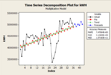
The time series plot above decomposed the data into four parts and enabled the team to evaluate the trend as well as seasonality.

In order to smooth out short-term fluctuations in the data and highlight the longer-term trends and cycles, the team averaged consecutive observations in the series to compute moving averages. Because the individual data points created by seasonality, cycles, and random variation are approximated in this model, the smoothed data set can reveal important patterns that would otherwise be difficult to spot.

The team gained yet another perspective by displaying the data using the single exponential smoothing method, which assigns exponentially decreasing weights to data points over time. This technique forecasted the plant’s electricity consumption in a way that placed greater emphasis on the more recent data.

Because single exponential smoothing is not ideal when there is a trend in the data, the project team introduced a second component using the double exponential smoothing method, which takes into account the possibility of a trend in the series. This approach also gives decreasing weights to older observations in the times series, but then smooths the trend and slope by using different constants for each.

In order to extend the double exponential smoothing method to include trend and seasonal variations, the team used a technique known as Winter’s method to calculate dynamic estimates for three components: level, trend, and seasonality.

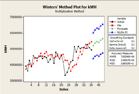
The Winters’ method plot, above, accounts for trend and seasonality in the series.

The variety of forecasting and smoothing methods offered in Minitab allowed the project team to easily analyze, display, and evaluate their data using each of these different approaches, as well as the method that incorporated their own plant-specific factors. The accuracy of each method was assessed by comparing each model’s results to actual data.

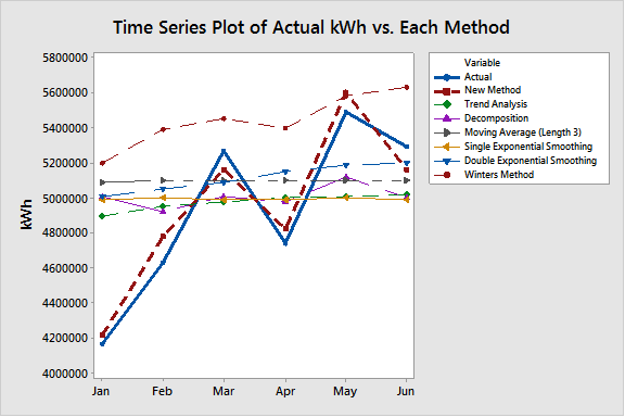
The time series plot above compares the plant’s actual kWh consumption over a six-month period with the forecasted energy usage of each model for the same period. The series for the actual consumption data and the forecasts for the project team’s new method are highlighted for comparison.

The forecasting method devised by the team incorporated specific factors relevant to the semiconductor plant’s process—such as machine requirements, machine idle time, and kilowatts used for each state—and adjusted the raw electricity usage data provided by the utility company. The team then compared the results of each established model to those of their own method.